Interactive Maps in Python, Part 3

Camera, lights, action! In this final part of our python cartography tutorial we take what we learned in part 1 and part 2 and set it in motion.

I might be biased by my personal attraction to things that move, but I think movement can bring data to life in a way nothing else can. We are still using trip data from the New York City bike share program. The movies we create in this tutorial will show the heartbeat of New York City. We will even drill down deep enough to see the individual trips progress. (If you want to see the end result, scroll down to the end of this post). As always, you can follow along with the jupyter notebook or get the source on github.

As before, we will use python and folium. Though folium has the capability of showing videos in a browser, we will only export our animations to separate video files.

Initial setup

Let’s start with some prerequisites. The seleniumpackage in python gives us access to a ‘headless’ browser. We will use selenium to automate the rendering of our maps and save them to a file.

pip install selenium

Update Nov 2018: Since selenium deprecated phantom.js we will use geckodriver instead. This also means we need to get the latest version of folium from their git repo.

pip install --upgrade git+https://github.com/python-visualization/folium

You’ll also need to download geckodriver and ffmpeg. For geckodriver you just have to extract the archive you downloaded and place the geckodriver file somewhere in your system PATH. This can be any folder on your system, and we can use python to set the PATH variable temporarily. For example, if we put the file in the same folder as the jupyter notebook, we would do:

import os
os.environ["PATH"] += os.pathsep + "."

In the previous tutorials, we wrote a lot of useful code so I moved some of those functions to a separate file called “consolidated_functions.py”, you can get it here. We import it under the name cf.

import consolidated_functions as cf

Now, on to the more exciting part!

Generating frames

The first challenge we run into is that we want to generate movies that vary smoothly in time. This means that we have to generate a sufficiently large number of frames over the (real-world) time span that we want to visualize. Option one is to aggregate the bike data into smaller time intervals, say, every minute. The problem with that approach is that there is a loss of variation in the number of arrivals at each station from minute to minute.

Therefore, we will take a different approach: we will still aggregate by hour but we will interpolate values for intermediate times.

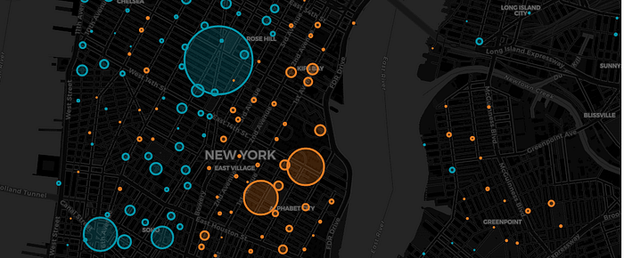
We can now generate a map corresponding to a desired time of day (specified as a float). We call the plot_station_countsfunction we wrote in part 1.

data = get_trip_counts_by_minute(9.5, bike_data)
cf.plot_station_counts(data, zoom_start=14)

The output should look this this:

We want to create many of these maps in a loop for different times of day. To do that, we need to write a function that takes some settings as input and saves one frame of the movie as an image file. Just before we save the frame to an image file, we also have the opportunity to add some annotations, such as a title and a timestamp. We use Pillow for that, just as we did in part 2. We’ll need to choose and download a font. Have a look at the google font book if you want some inspiration. We will be using Roboto light.

Next, we generate a sequence of these frames that we can stitch together into a movie. We call our function in a loop to generate many frames.

for i, hour in enumerate(np.arange(6, 23, .2)):
    go_frame(i, hour, save_path="frames")

This process can be pretty time consuming, you could look into using the multiprocessingpackage in python (look for Pool.map()).

Fixing missing tiles

The tiles for the background maps are loaded from the web for each frame. Due to the way the frames are rendered, you may see some gray blocks in your frames when the tiles failed to load in time. This can be remedied by regenerating the affected frames. For example, like this:

arrival_times = np.arange(6, 23, .2)
frames_to_redo = [27, 41, 74, 100, 105]
for i in frames_to_redo:
    hour = arrival_times[i]
    go_arrivals_frame(i, hour, "frames")

This issue will be addressed in the next release of folium by introducing a delay argument to the _to_png() function.

Stitching frames into movies

We can convert the resulting images into a movie using ffmpeg (or your favorite video editing program). We will do this from the command line like this:

ffmpeg -r 10 -i frames/frame_%05d.png -c:v libx264 -vf fps=25 -crf 17 -pix_fmt yuv420p output.mp4

You may have to specify the full path to ffmpeg if the executable is not on your system PATH.

I’ll leave it as an exercise to do the same thing for the maps of paths we created in part 2. (but be sure to checkout the jupyter notebook if you’re interested in the answer). Here is the final result.

Learned something? Click the 👏 to say “thanks!” and help others find this article.